Relationships among many variables
Data Computing
November 16, 2016
We have spent most of our time on two subjects:
- Data visualization
- Data wrangling: getting from the data you are given to the “glyph-ready” data that you need to make a graphic or some other mode to guide interpretation of the data.
Visualization works well with 1-3 variables, and in some situations can work with more variables.
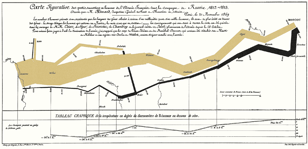
A multivariable graphic
Glyph: geom_path() or “Sankey”, Annotations: rivers and towns
Aesthetics: (x,y) latitude and longitude; size size of army; color advance or retreat.
source
A multivariable graphic in R

Not bad! …although I don’t blame you if you prefer Charles Minard to ggplot2
p.s. I can’t take credit for most of the code; I did the same thing I often recommend you do:
- Google search
- start with working code that does something similar
- tweak it until it does what you want. (it didn’t need much)
With more variables?
If we need to relate more variables, a visualization may not suffice.
Formal mathematical representations provide an alternative:
- model formulas, e.g.
lm()
- other structures for models, e.g. regression or classification trees.
Example: Child carseat sales
Purpose: Figure out how to raise sales of a brand of carseats.
head(ISLR::Carseats %>% rename(CompP=CompPrice, Ads=Advertising, Pop=Population,
                               Shelf=ShelveLoc, Edu=Education))
| 9.50 |
138 |
73 |
11 |
276 |
120 |
Bad |
42 |
17 |
Yes |
Yes |
| 11.22 |
111 |
48 |
16 |
260 |
83 |
Good |
65 |
10 |
Yes |
Yes |
| 10.06 |
113 |
35 |
10 |
269 |
80 |
Medium |
59 |
12 |
Yes |
Yes |
| 7.40 |
117 |
100 |
4 |
466 |
97 |
Medium |
55 |
14 |
Yes |
Yes |
| 4.15 |
141 |
64 |
3 |
340 |
128 |
Bad |
38 |
13 |
Yes |
No |
| 10.81 |
124 |
113 |
13 |
501 |
72 |
Bad |
78 |
16 |
No |
Yes |
Hypothesis generated model
- Price relative to competitor’s price is relevant.
- Larger population gives larger sales
- Education level?
- Advertising?
Carseats <-
  ISLR::Carseats %>%
  mutate(rel_price = Price / CompPrice)
mod1 <-
  Carseats %>%
  lm(Sales ~ rel_price + Population + Education + Advertising,
     data = .)
coef(mod1)
##   (Intercept)     rel_price    Population     Education   Advertising
##  17.497352098 -10.907759402  -0.000139262  -0.055051345   0.136911760
Interpreting the model?
##
## Call:
## lm(formula = Sales ~ rel_price + Population + Education + Advertising,
##     data = .)
##
## Residuals:
##    Min     1Q Median     3Q    Max
## -6.005 -1.470 -0.118  1.310  5.280
##
## Coefficients:
##               Estimate Std. Error t value Pr(>|t|)
## (Intercept)  1.750e+01  8.728e-01  20.048  < 2e-16 ***
## rel_price   -1.091e+01  6.673e-01 -16.345  < 2e-16 ***
## Population  -1.393e-04  7.470e-04  -0.186    0.852
## Education   -5.505e-02  4.051e-02  -1.359    0.175
## Advertising  1.369e-01  1.651e-02   8.294 1.74e-15 ***
## ---
## Signif. codes:  0 '***' 0.001 '**' 0.01 '*' 0.05 '.' 0.1 ' ' 1
##
## Residual standard error: 2.108 on 395 degrees of freedom
## Multiple R-squared:  0.4483, Adjusted R-squared:  0.4427
## F-statistic: 80.25 on 4 and 395 DF,  p-value: < 2.2e-16
No prior model at all?
mod3 <- Carseats %>% rpart(Sales ~ ., data=.)
prp(mod3)

Shelf location?
mod4 <- Carseats %>%
  rpart(Sales ~ rel_price + Advertising + ShelveLoc + Population, data=.)
prp(mod4)

Unsupervised learning
Dists <- dist(mtcars)
Dendrogram <- hclust(Dists)
ggdendrogram(Dendrogram)

Important Machine Learning concepts
- Cross-validation
- Supervised vs unsupervised learning
- Recursive partitioning
- Dimension reduction
Activity: Supervised Machine Learning
Grading
The assignment is worth a total of 10 points.

